Below are images I shot so the transforms between them are projective so I can create image mosaics using them. I chose images at School of Law, Haas, and South Hall.
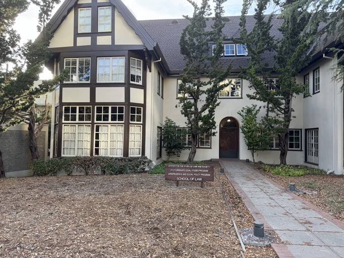
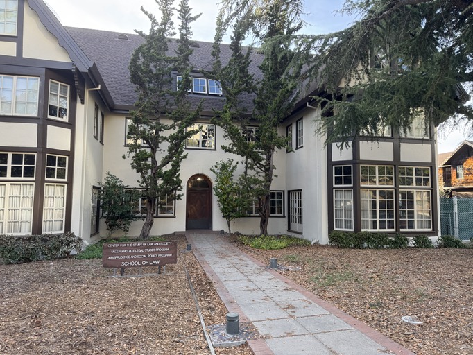
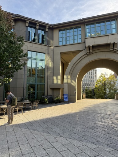
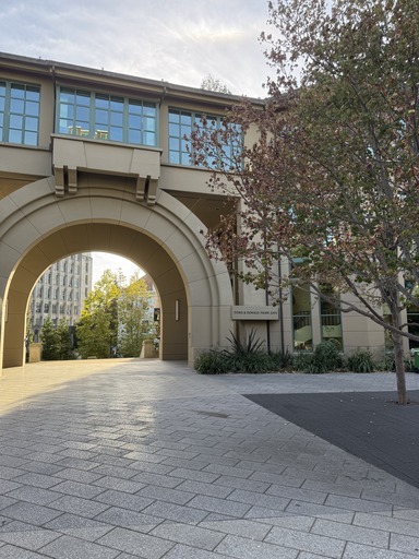
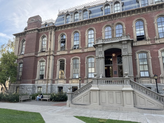
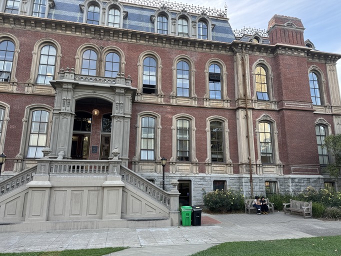
We can represent the projective transformation between each left and right image using a homography matrix, \(H\), Our projective transformation can be written as \(Hp = p'\). Where \(p\) is a homogeneous coordinate of a point in the left image, and \(p'\) is its corresponding point in the right image. $$ H = \begin{bmatrix} a & b & c \\ d & e & f \\ g & h & 1 \end{bmatrix} $$ The projective transformation is as follows: $$ \begin{bmatrix} a & b & c \\ d & e & f \\ g & h & 1 \end{bmatrix} \begin{bmatrix} x_1 \\ y_1 \\ 1 \end{bmatrix} = \begin{bmatrix} wx_1' \\ wy_1' \\ w \end{bmatrix} $$ Using our corresponding pairs of points we can recover the homography, \(H\), by solving the following system using least squares. We stack each correspondence pair in a matrix, \(P\), on the left, and a vector \(q\) on the right. Since we have 8 degrees of freedom, we need at least 4 points. $$ \begin{bmatrix} x_1 & y_1 & 1 & 0 & 0 & 0 & -x_1'x_1 & -x_1'y_1 \\ 0 & 0 & 0 & x_1 & y_1 & 1 & -y_1'x_1 & -y_1'y_1 \\ \end{bmatrix} \begin{bmatrix} a \\ b \\ c \\ d \\ e \\ f \\ g \\ h \end{bmatrix} = \begin{bmatrix} x_1' \\ y_1' \end{bmatrix} $$
After we recovered the homography, \(H\), we want to be able to warp images using it. To do this we take the corners of the image we would like to warp and apply H to get the tranformed coordinates on the warped image. We do this as follows: $$ \begin{bmatrix} a & b & c \\ d & e & f \\ g & h & 1 \end{bmatrix} \begin{bmatrix} x_1 \\ y_1 \\ 1 \end{bmatrix} = \begin{bmatrix} wx_1' \\ wy_1' \\ w \end{bmatrix} $$ $$ warped\ pixel\ location = \begin{bmatrix} \frac{x_1'}{w} \\ \frac{y_1'}{w} \end{bmatrix} $$ Afterwards, we create a bounding box in the warped image that contains these morphed corners. We use inverse warping to determine what these pixels would be in the original images and use interpolation to set these pixels in our warped image.
To test if our warp works lets try to "rectify" some images by selecting a planar surface of an image and projecting it onto a flat frontal-facing plane. Here are the results below:
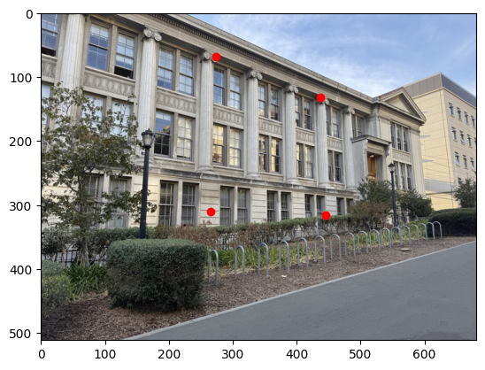
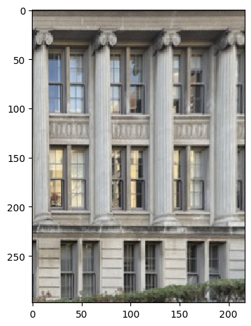
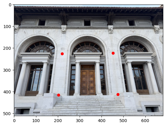
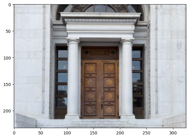
We see the surfaces we chose have been warped to be frontal-facing.
After we project the left image into the right images space, we need to blend the two images together. We can do this using 2-band "laplacian stack" blending. First, we create a mask of where the projected images are on our blending canvas that will encompass both images. After we create these masks, we apply a distance transform to find the distances of pixels in the mask to their nearest edge and then normalize these distance values from 0 to 1 for both images.
Here are the results of this step on the School of Law left and right images:
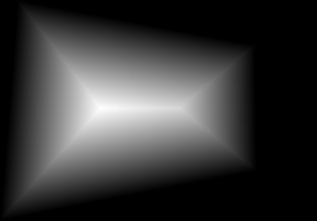
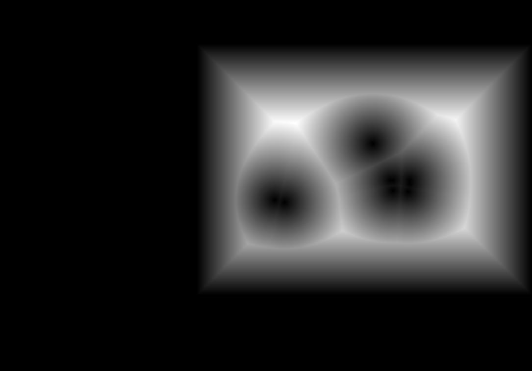
Now we apply a low-pass filter and a high-pass filter on the left and right images. We blend the low-pass and high-pass left and right images separately and sum them to create our blended images. To blend the low-pass filtered images we apply a weighted linear combination on the left and right images using the distance transformed computed above. To blend the high-pass filtered images we just selected the pixel from the image that has a greater distance value in each image.
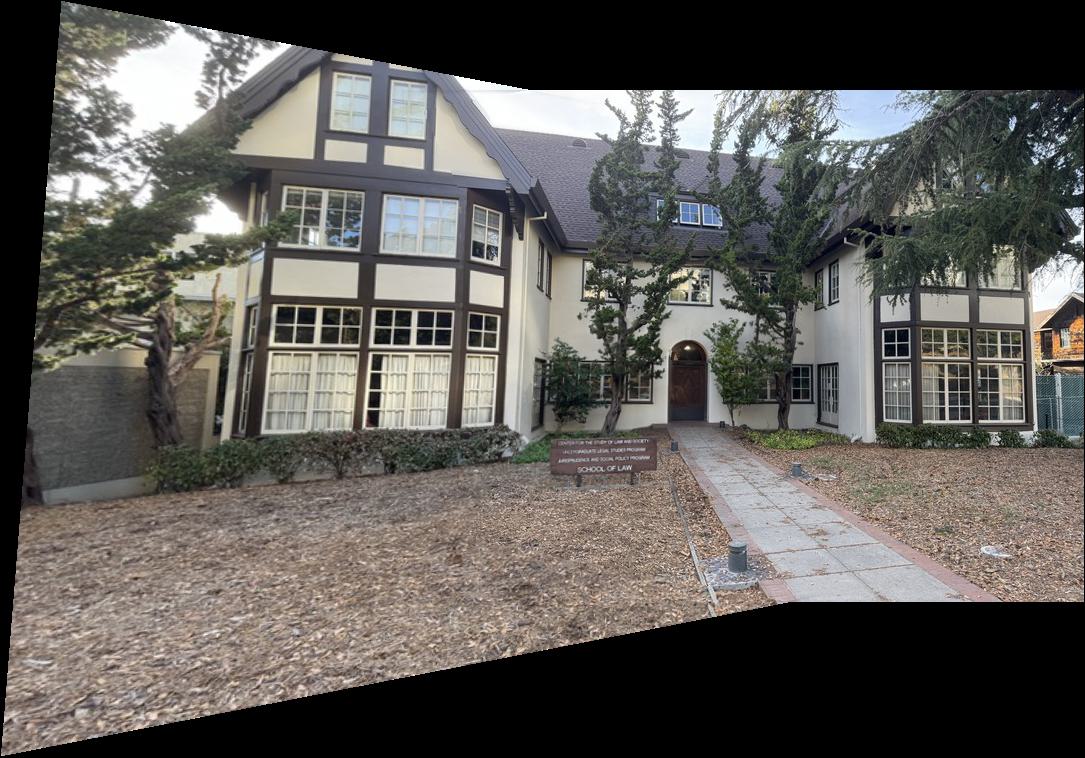
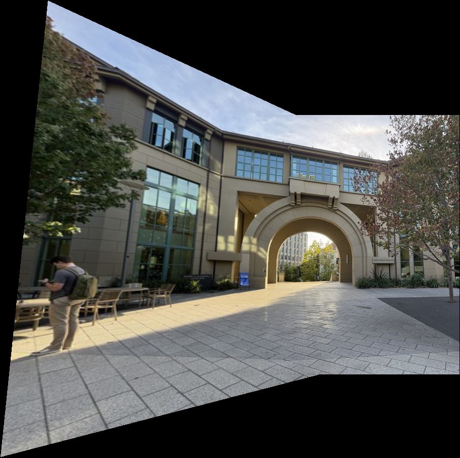
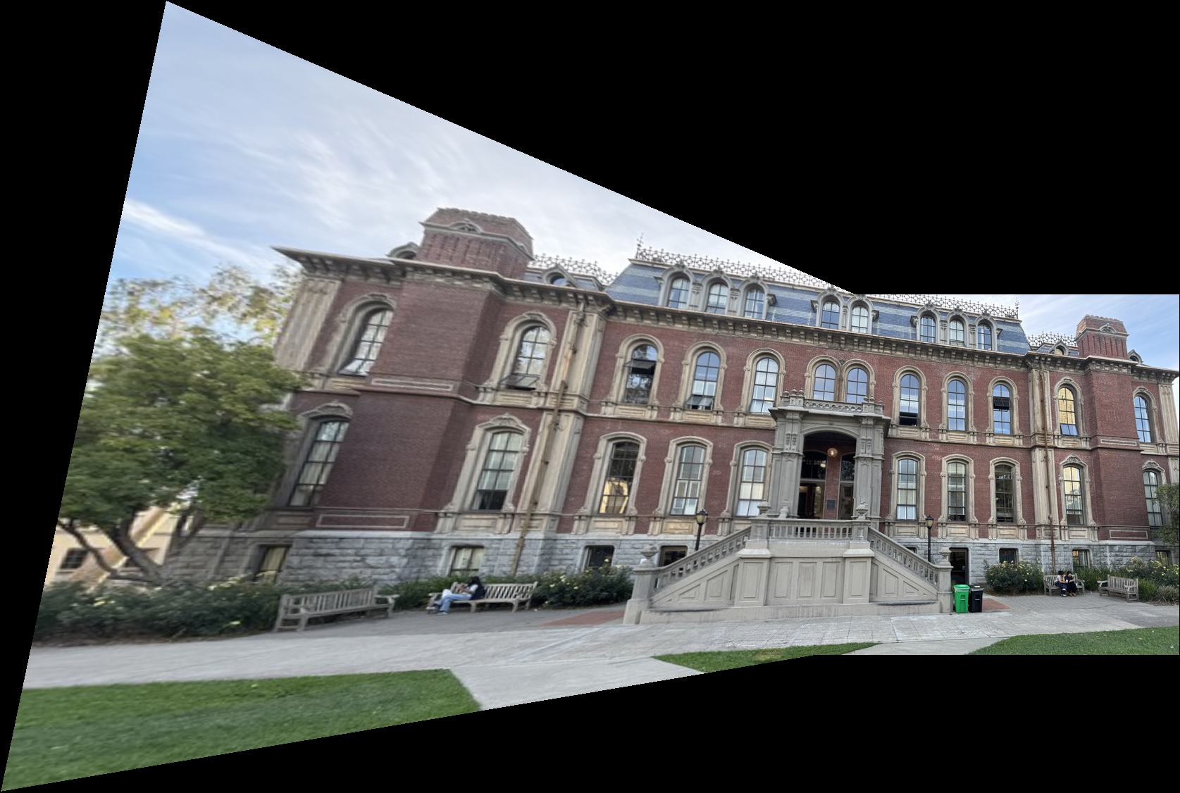
Here are the results of the mosaics using the images chosen from the Shooting the Pictures section:
For autostitching, we want to first create a set of interest points to use.
To create this initial set of interest points we can use the Harris Interest Point
Detector. We can use the Harris Interest Point Detector to get a matrix of "corner
strengths" representing the strength of the interest points in the image and set of
interest points to use.
Applying the detector below we get the following set of interest points for a sample
image:
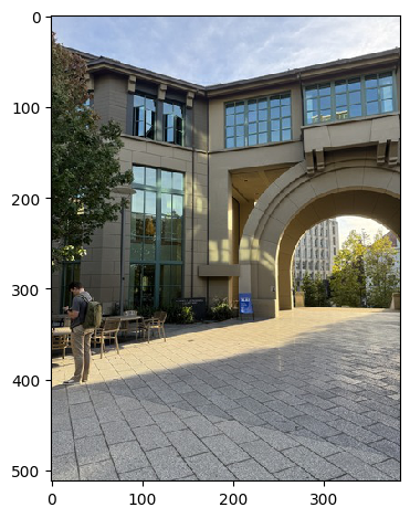
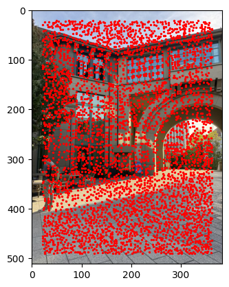
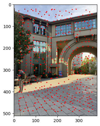
We see that the Harris interest points are clustered together and not evenly spaced throughout the image. We can run adaptive non-maximal suppression to select interest points with strong corner reponse that are spaced through the image. For each interest point we compute the radius as follows: $$ r_i = \min_j |\mathbf{x}_i - \mathbf{x}_j|, \text{ s.t. } f(\mathbf{x}_i) < c_{\text{robust}}f(\mathbf{x}_j), \mathbf{x}_j \in \mathcal{I} $$ We select the top k points with the largest radii to make up our set of evenly spread out interest points.
Setting k=500, here is the comparison of the Harris interest points and the points after running ANMS:

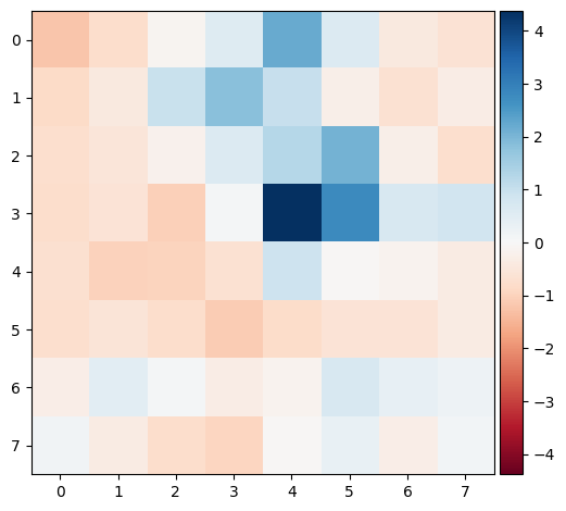
Once we have our finalized interest points, we want to extract features for each point. To do this we take a 40 x 40 window around each point. We then downsample using a scaling factor of 5 to create 8 x 8 patches. We bias/gain-normalize to have zero mean and unit variance. We then flatten the patch into a vector, giving us a feature descriptor for each interest point.
Below we have an example of normalized patch before it is flattened:
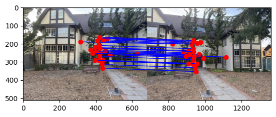
With the features extracted, we need to match features across our images to form correspondences. We first compute the distances between the two sets of feature descriptors we have for our two images. Then we iterate through our first set of descriptors and find the first and second nearest neighbor in the second set of descriptors. To reduce the number of outliers we use Lowe's trick and compute ratio of the first nearest neighbor distannce and the second nearest neighbor distance. If the ratio is below some threshold, \(t\), we then count the feature in first feature descriptor set as a match with its nearest neighbor in the second feature descriptor set.
Here are the feature matches for the School of Law using \(t = 0.1\):
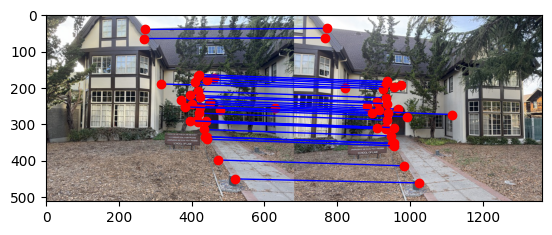
Even with Lowe's trick we are left with some incorrect feature matches. When we compute the homography using least squares
with these outliers we skew the compute homography, creating invalid stitching and warps.
In order to remove the amount of outliers we apply RANSAC to create a set of inliers to compute our homography.
The steps are as follows:
Here are our feature matches after running RANSAC on the School of Law images:
Here are the results comparing the hand-stitched mosaics versus the auto-stitched mosaics using feature matching and RANSAC:

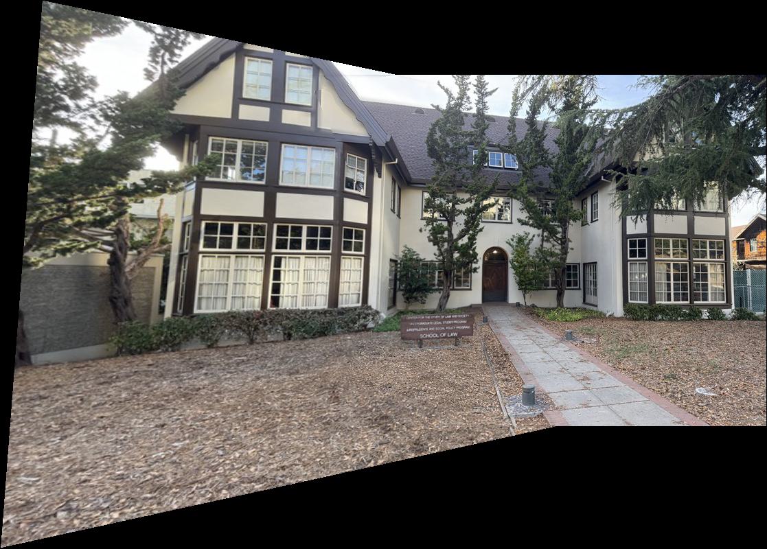

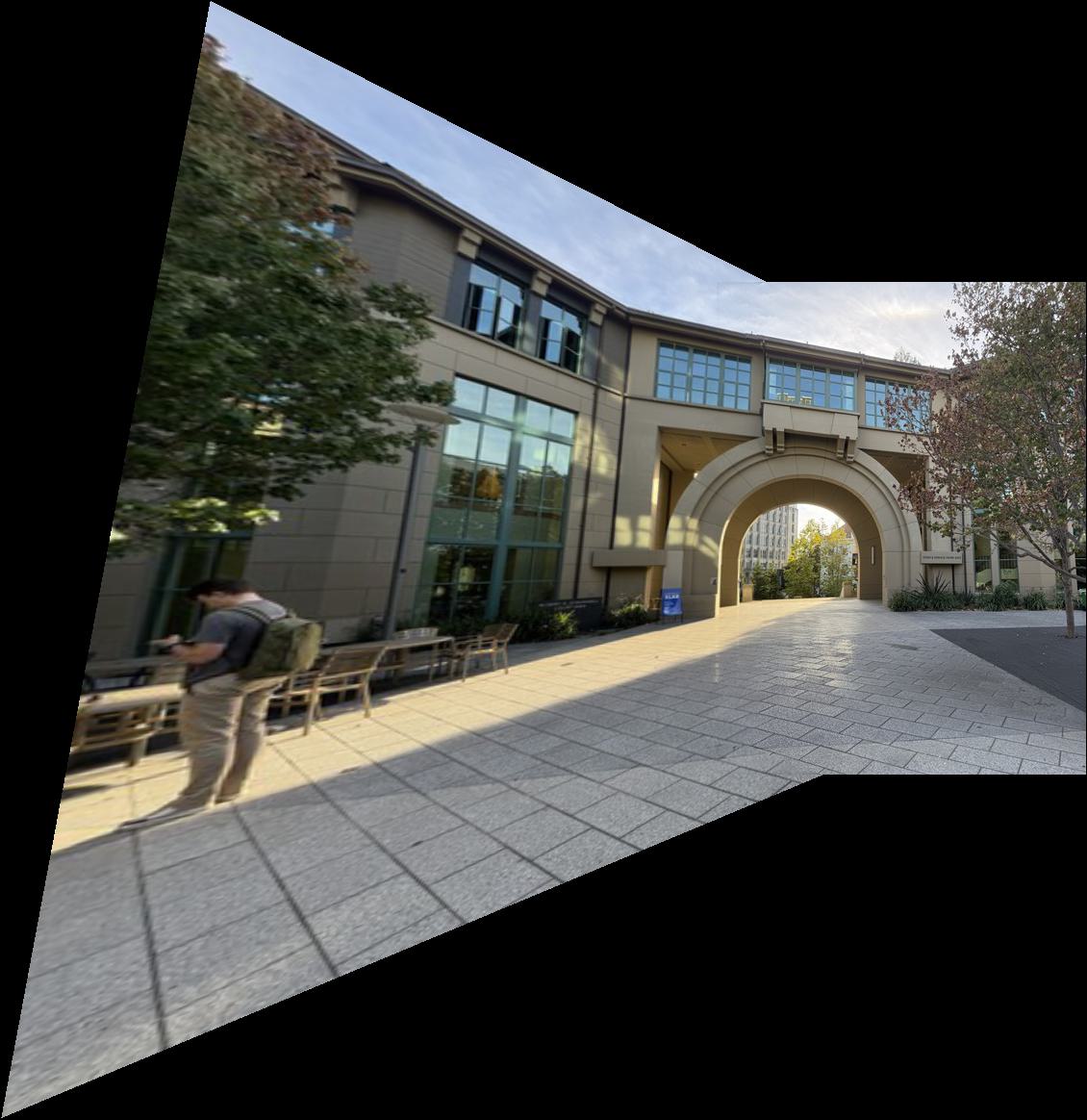

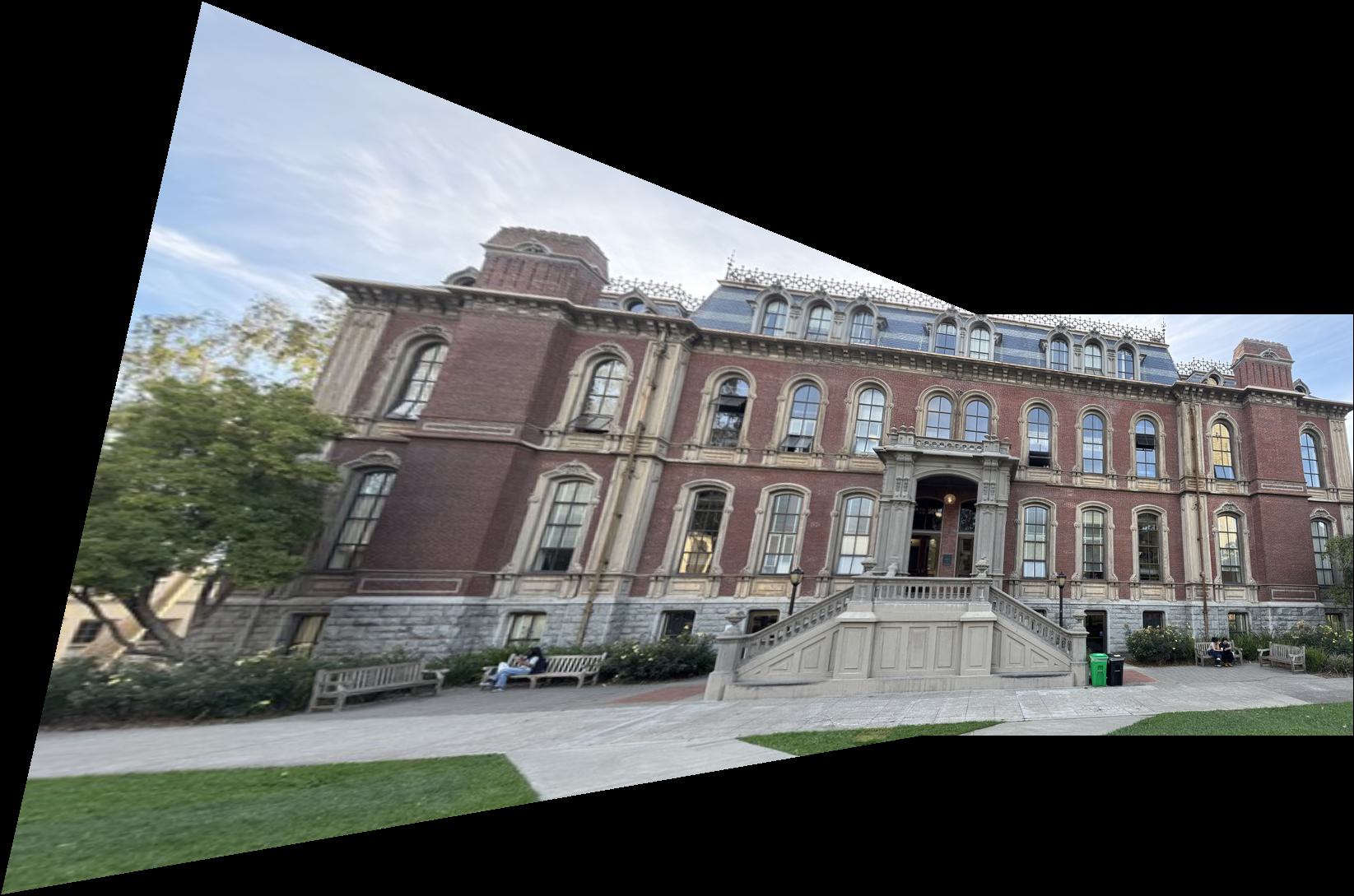
What I found particularly interesting and cool was Lowe's trick and RANSAC as a tool to mitigate incorrect correspondences and automatically chose the right ones to compute the homography.