Diffusion Models

Part A: The Power of Diffusion Models

Setup

To gain familiarity with diffusion models, we will use the DeepFloyd IF diffusion model trained by Stability AI. Let's look at the output of the model with a series of text prompts and different inference steps using a random seed of 180.

"An oil painting of a snowy mountain village"

"A man wearing a hat"

"A rocket ship"

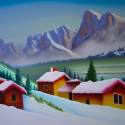
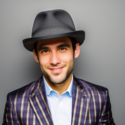
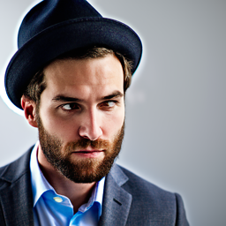
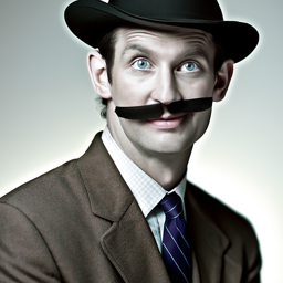
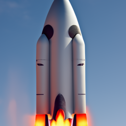
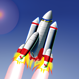
We see the prompts with more detail and specification like the "oil painting of a snowy mountain village" result in a higher quality image that's standardized across different inference steps. We also see that lower inference steps despite their speed come at the cost of reduced quality in the image generated.

Sampling Loops

In this section we will be using DeepFloyd's denoisers to implement sampling loops that generate high-quality images. To sample and generate images using these models we start with pure noise at some timestep \(T\), sampled from a Gaussian distribution giving us \(x_T\). Using a diffusion model like DeepFloyd, we can reverse this process by predicting and removing the noise at each timestep t, until we get a clean image \(x_0\). We can use these and modify these sampling loops for a variety of tasks like inpainting or creating optical illusions.

Implementing the Forward Process

The forward process is a fundamental aspect of diffusion models. It takes a clean image and adds noise to it as follows: $$x_t = \sqrt{\bar{\alpha_t}}x_0 + \sqrt{1-\bar{\alpha_t}}\epsilon \text{ where } \epsilon \sim N(0,1)$$ We use the alphas_cumprod variable, \(\bar{\alpha_t}\), which contains the noise coefficients from the DeepFloyd model for our forward pass.

Below are the results at different noise levels for the Campanile:

Classical Denoising

Let's attempt to denoise our images using classical methods like Gaussian blur filtering.

Here are the results below:

One-Step Denoising

We see classical denoising was ineffective in the removing the noise. Let's try using the pretrained diffusion to remove the noise using one-step denoising.

Iterative Denoising

We saw the one-step denoising was effective compared to the Gaussian blur filtering. However, diffusion models are designed to denoise iteratively. We can iterate over a series of timesteps starting off at the largest \(t\) corresponding to the noisest image to the smallest \(t\) corresponding to the clean image. At each timestep we apply the following formula: $$x_{t'} = \frac{\sqrt{\bar{\alpha_t}}\beta_t}{1-\bar{\alpha_t}}x_0 + \frac{\sqrt{\alpha_t}(1-\bar{\alpha_t})}{1-\bar{\alpha_t}}x_t + v_\sigma$$

where:

• \(x_t\) is your image at timestep \(t\)
• \(x_{t'}\) is your noisy image at timestep \(t'\) where \(t' < t\)
• \(\bar{\alpha}\) is defined by alphas_cumprod
• \(\alpha_t = \frac{\bar{\alpha_t}}{\bar{\alpha_{t'}}}\)
• \(\beta_t = 1 - \alpha_t\)
• \(x_0\) is our current estimate of the clean image
• \(v_0\) is random noise

Here are the results below:

Diffusion Model Sampling

Previously, we used the diffusion model to denoise images. However, we can also use it to generate images from scratch.

Here are some samples:

Classifier-Free Guidance (CFG)

To improve the quality of the images generated at the expense of image diversity, we can use classifier-free guidance. We compute a conditional and unconditional noise estimate. These are denoted as \(\epsilon_c\) and \(\epsilon_u\). We then use the following noise estimate: $$\epsilon = \epsilon_u + \gamma(\epsilon_c - \epsilon_u)$$ \(\gamma\) controls the strength of CFG. When \(\gamma\) > 1, we get higher quality images.

Below are generated images using CFG:

Image-to-Image Translation

We can use varying noise levels to make edits to existing images. The more noise in image the greater the edits to the existing image will be. We're going to take our test images, noise them, and force them back into the image manifold without any conditioning. This will result an image similar to our original image depending on the noise level we start at. This approach follows the SDEdit algorithm.

Here are the results below:

Editing Hand-Drawn Images and Web Images

The procedure above works well if we start with nonrealistic images and then project onto the natural image manifold. Let's try with hand drawn and web images.

Here are the results:

Inpainting

We can use diffusion models to implement inpainting. Given an image \(x_{orig}\) and a binary mask \(\textbf{m}\), we can create a new image. This new image will have the same content as the original where \(\textbf{m}\) is 0 and new content where \(\textbf{m}\) is 1.

At every step of the diffusion denoising loop we apply the following formula: $$x_t \leftarrow \mathbf{m}x_t + (1-\mathbf{m})\text{forward}(x_{orig}, t)$$

Here are the results:

Text-Conditional Image-to-Image Translation

We can also use different text prompt to guide the projection in image-to-image translation, giving us control via language.

Here are the results below using different prompts:

"A rocket ship"

"A photo of the amalfi coast"

"An oil painting of a snowy mountain village"

Visual Anagrams

Using our diffusion model, we can create optical illusions like visual anagrams. We can create images that like look one way right-side up, and like another flipped upside down. To do this we run the denoising step on the following noise estimate: $$\epsilon_1 = UNet(x_t,t,p_1)$$ $$\epsilon_2 = flip(UNet(flip(x_t),t,p_2))$$ $$\epsilon = (\epsilon_1 + \epsilon_2)/2$$

where:

• UNet is the diffusion model
• flip is a function that flips the image
• \(p_1\) and \(p_2\) are 2 different text prompt embeddings
• \(\epsilon\) is our final noise estimate

Here are the results:

Hybrid Images

Using our diffusion model, we can create hybrid images. Hybrid images that like look one way from up close, and like another image from far away. To do this we run the denoising step on the following noise estimate: $$\epsilon_1 = UNet(x_t,t,p_1)$$ $$\epsilon_2 = UNet(x_t,t,p_2)$$ $$\epsilon = f_{lowpass}(\epsilon_1) + f_{highpass}(\epsilon_2)$$

where:

• UNet is the diffusion model
• \(f_{lowpass}\) is a low pass function
• \(f_{highpass}\) is a high pass function
• \(p_1\) and \(p_2\) are 2 different text prompt embeddings
• \(\epsilon\) is our final noise estimate

Here are the results:

Part B: Diffusion Models from Scratch!

Training a Single-Step Denoising UNet

Let's start by building a simple one-step denoiser. Given a noisy image \(z\), we aim to train a denoiser \(D_{\theta}\) such that it maps \(z\) to a clean image \(x\). To do so, we can optimize over an L2 loss: $$ L = \mathbb{E}_{z,x}||D_{\theta}(z) - x||^2 $$

Implementing the UNet

We implement the UNet according to the following diagrams:

Using the UNet to Train a Denoiser

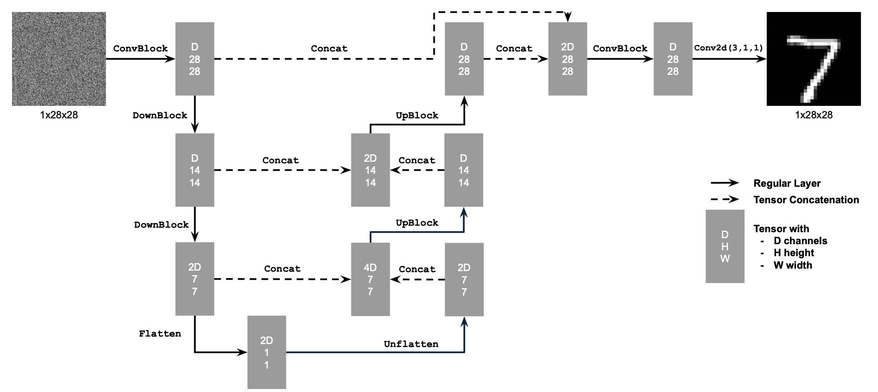
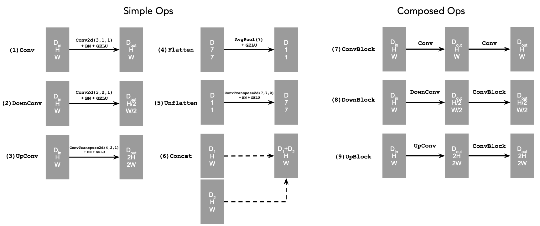
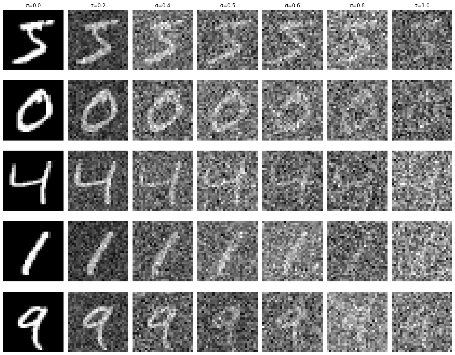
To train our denoiser, we need to generate training data pairs of \((z, x)\), where \(x\) is a clean MNIST digit. For each training batch, we generate \(z\) from x using the following formula: $$z = x + \sigma\epsilon, \quad \text{where } \epsilon \sim N(0, I)$$

Here's a visualization of the noising process:

Training

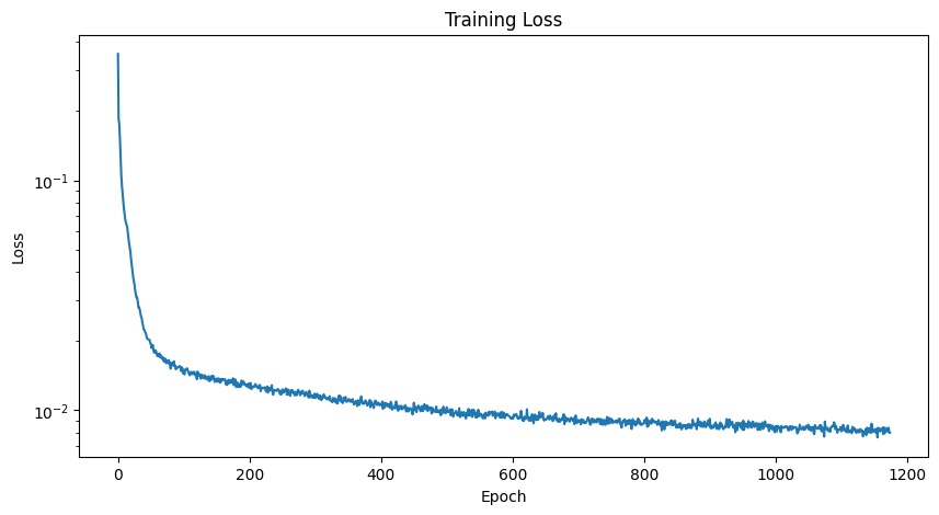
Now let's train our model to perform denoising. Below is the training losses curve:

Here are the results following the 1^st and 5^th epochs:

Out of Distribution Testing

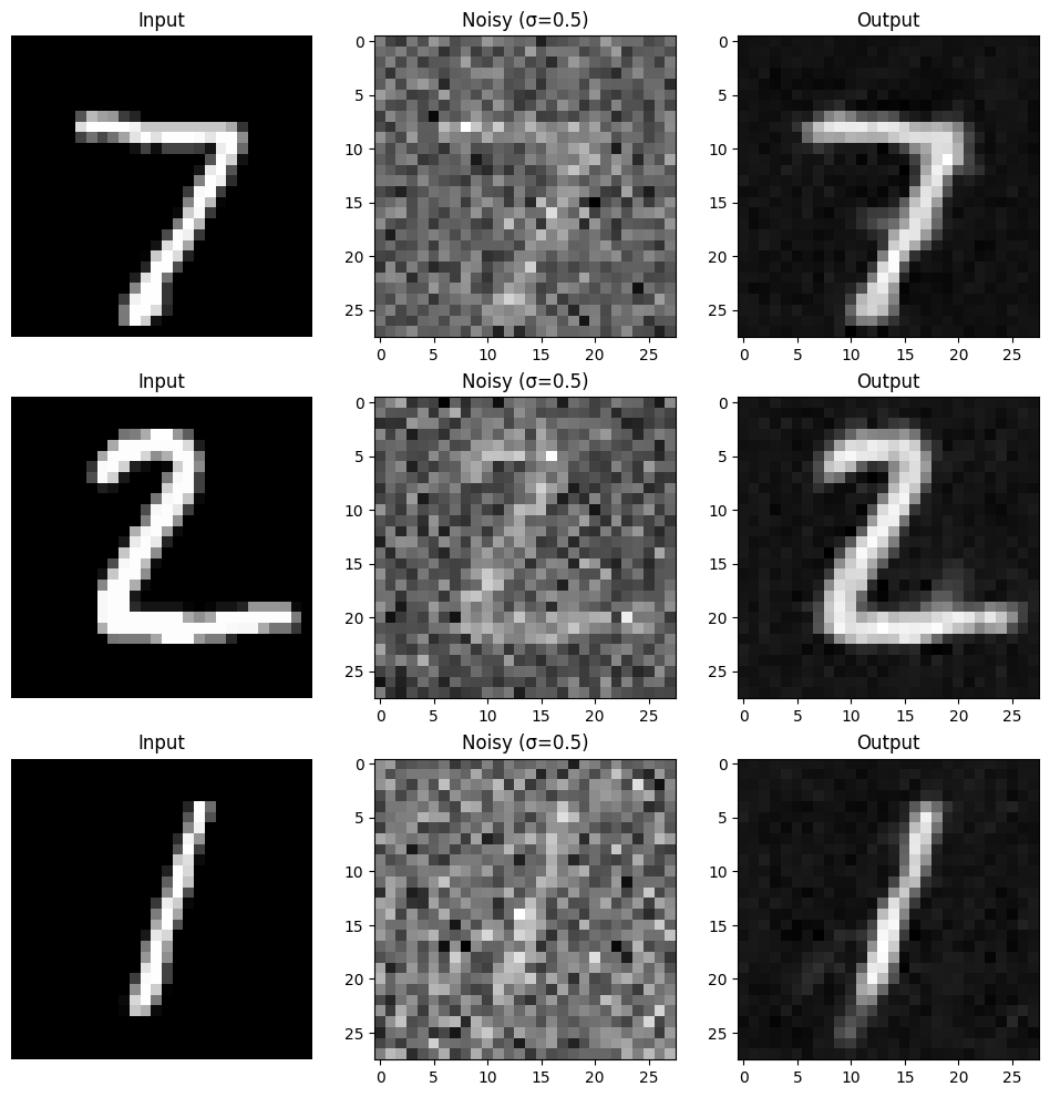
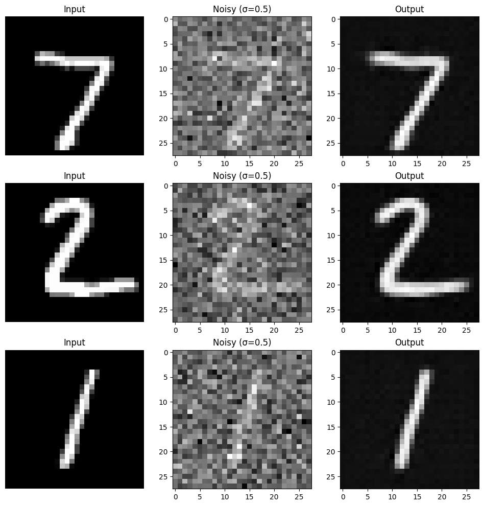
The model was trained with MNIST digit values with \(\sigma=0.5\). Let's see how the model performed with other sigma values.

Here are the results:

Training a Diffusion Model

Now we can use diffusion and train a UNet model to iteratively denoise images using the DDPM approach.

Instead of predicting the clean image directly, our UNet now predicts the noise that was added. For a noisy image \(z\), our objective function becomes:

$$ L = \mathbb{E}_{\epsilon}||e_{\theta}(z) - \epsilon||^2 $$

For diffusion, we follow a gradual process where we start with pure noise sampled from \(N(0, I)\). We then iteratively denoise the image using timesteps \(t \in \{0, 1, \cdots, T\}\). Finally, we generate noisy images at each timestep using the following equation:

$$ x_t = \sqrt{\bar{\alpha_t}}x_0 + \sqrt{1-\bar{\alpha_t}}\epsilon \quad \text{where } \epsilon \sim N(0,1). $$

We construct \(\bar{\alpha_t}\) as follows:

• \(\beta\) is a list of length \(T\) that starts at 0.0001 and ends at 0.02 with values evenly spaced between the two
• \(\alpha_t = 1 - \beta_t\)
• \(\bar{\alpha_t} = \prod_{s=1}^t \alpha_s\) is a cumulative product of \(\alpha_s\) for \(s \in \{1, \cdots, t\}\).

To denoise \(x_t\) we apply the UNet on it to get \(\epsilon\). We can condition on t since the variance of \(x_t\) varies with \(t\), giving us the our final objective function: $$L = \mathbb{E}_{x_t,t}||e_{\theta}(x_t, t) - \epsilon||^2$$

Adding Time Conditioning to UNet

We add time conditioning to our UNet model using the following diagrams:

Training the UNet

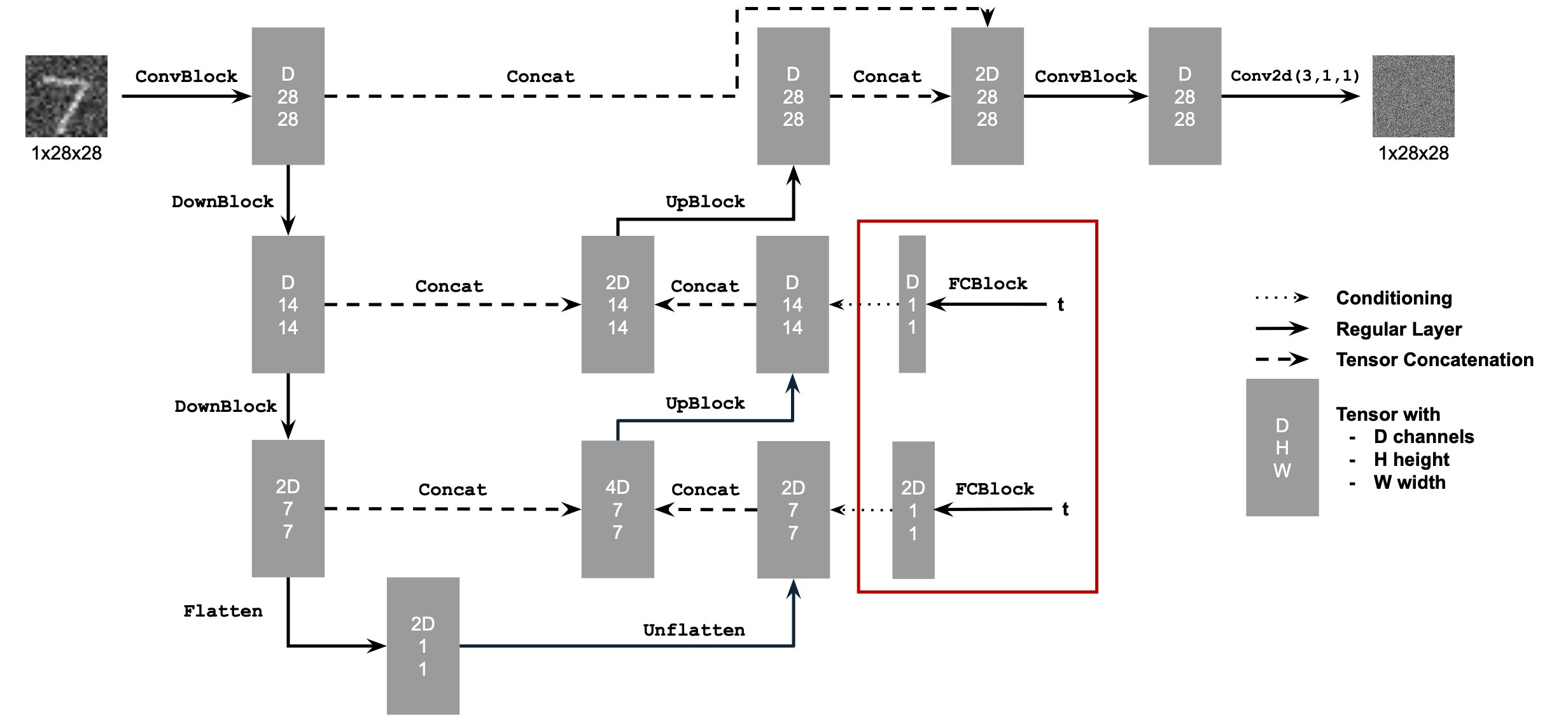
We train the time-conditioned UNet using the following algorithm:

Here are the training losses:

Sampling from the UNet

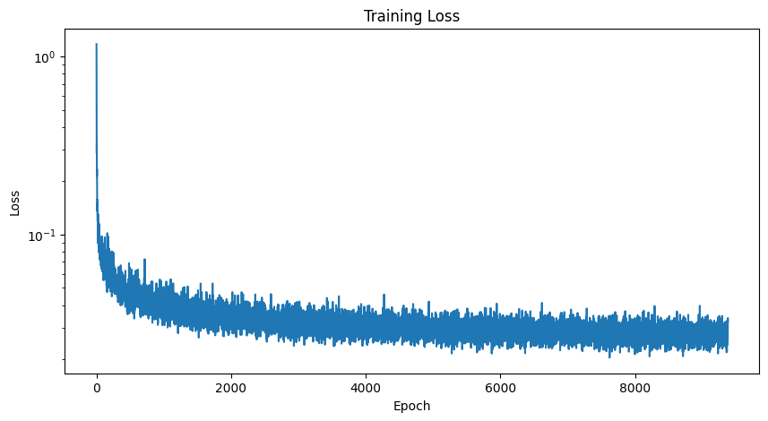
We sample from the time-conditioned UNet using the following algorithm:

Here are the results following the 5^th and 20^th epochs:

Adding Class-Conditioning to UNet

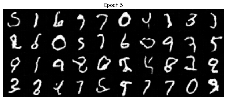
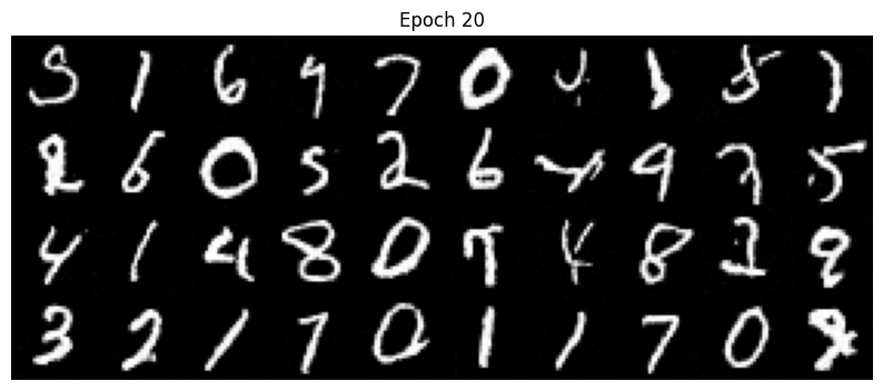
To make the results better and give us more control for image generation, we can also condition our UNet on the class of the digit 0-9. This will require adding 2 more FCBlocks to our UNet that take in a class-conditioning vector \(c\) that one-hot encodes the digit. To ensure our UNet works without being conditioned on teh class, we implement dropout 10% of the time.

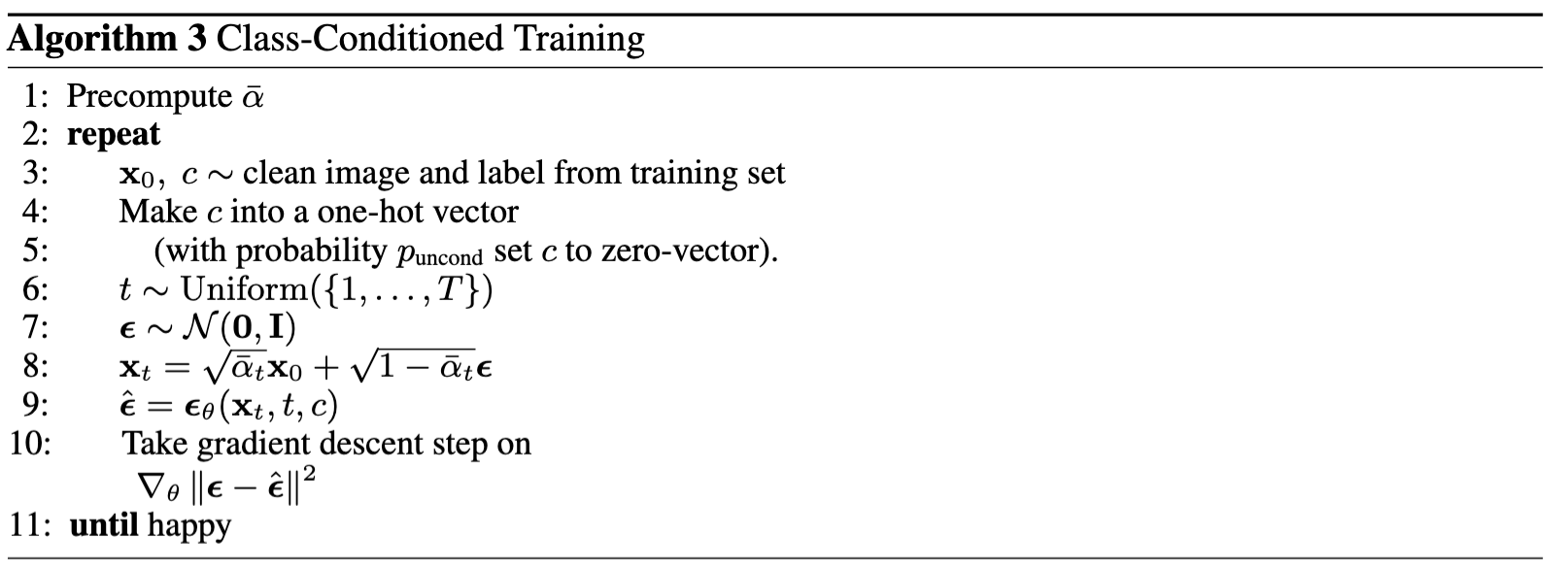
To train the class-conditioned UNet we apply the following algorithm:

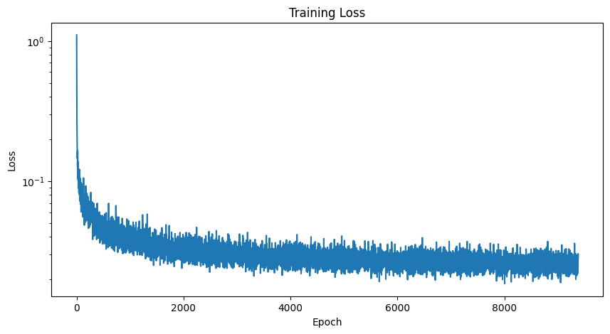
Here are the training losses:

Sampling from the Class-Conditioned UNet

We sample from our class-conditioned UNet as follows:

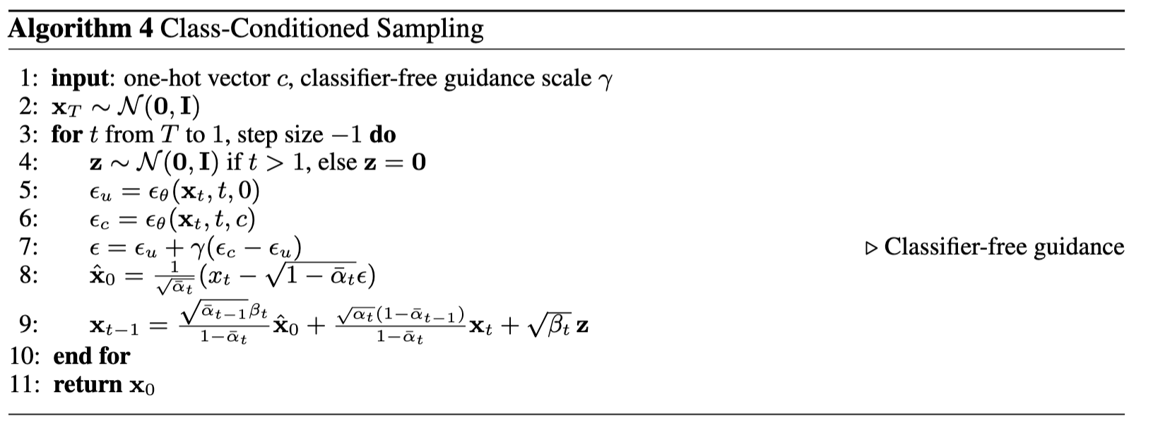
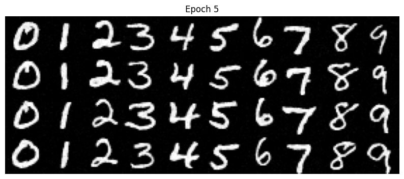
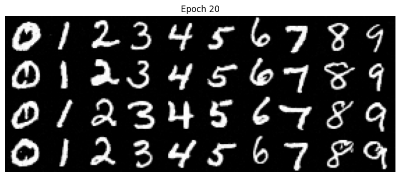
Here are the results following the 5^th and 20^th epochs: